Team Members
- Graham Schock
- Jonathan Lee
- Jack Umina
Single Scale Alignment
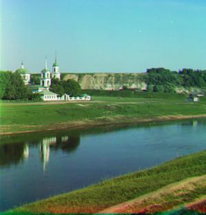
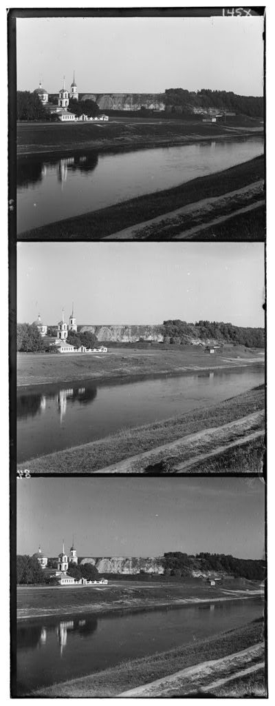
In this project we want to take three different color channels of the same image and align them together. Consider the following three channels of the same image:
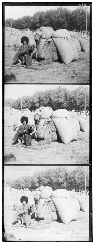
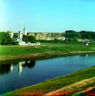
We want to transform these 3 channels into one color image by finding the correct way to align all of the three images together. For example the three images given above would transform into 1 color image given below:
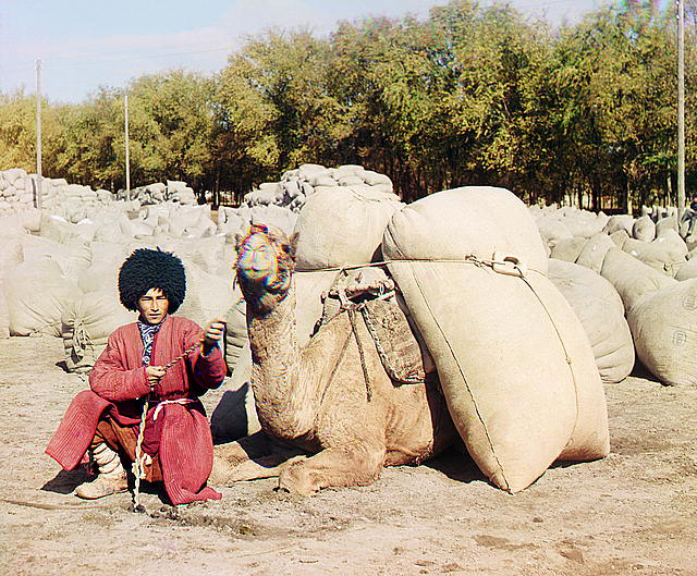
The above image was manually aligned and altered to achive the correct image. We want a way to automate this process by checking image similarity for a range of alignments.
Implementation
We can come up with a way to bruteforce this solution with the following algorithm along with some python code using scikit image:
- Divide the image into the three color channels
height = int(np.floor(im.shape[0] / 3.0)) b = im[:height] # Get blue g = im[height: 2*height] # Get green r = im[2*height: 3*height] # Get red - Take two of the three color channels (for example green and blue)
align(g, b) # Align green and blue -
Iterate through x and y displacements from [-15, 15]
- For each x and y displacement apply a transform to translate by the x and y to 1 of the channels
def apply_transform(chan, dispx, dispy): tform = transform.SimilarityTransform(scale=1, rotation=0, translation=(dispx, dispy)) chan = transform.warp(chan, tform) return chan - Calculate the similarity between the transformed channel and the untouched channel by using sum of squared difference
def score(chan1, chan2, dispx, dispy): chan1 = apply_transform(chan1, dispx, dispy) return np.sum(((chan1 - chan2) ** 2)) - Find the minimum sum of squared difference of all displacements and return that transform
def align(chan1, chan2): best = float('inf') best_disps = [float('inf'), float('inf')] for dispx in range(-15, 15): for dispy in range(-15, 15): cur_score = score(chan1, chan2, dispx, dispy) if cur_score < best: best = cur_score best_disps = [dispx, dispy] #print(best_disps) return apply_transform(chan1, best_disps[0], best_disps[1]) -
Do steps 2 - 6 for two other color channels (for example red and blue)
- stack all 3 of the channels together (for example: (aligned green and blue), (alligned red and blue) and untouched blue)
im_out = np.dstack([ar, ag, b])
skio.imsave(fname, im_out) # Print the image
Evaluation
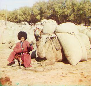
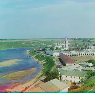
Consider the 3 color channels of the camel image. When we apply this algorithm to those color channels we get the following result:
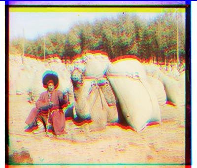
From running this algorithm we also saw that the optimal alignment was shifting each channel [0, -2].
While the image is blurry with many artifacts we see that the colors presented in the image do make sense. For example the sand is yellow and the trees are green.
It was also evident that the borders could be messing up our alignment so we pursued automatic cropping as an extra feature which led to a lot better image (will be presented later).
We also noticed that it took too long to run on the higher definition images, so we will present those in the next section.
Multi Scale Alignment
Greedy Algorithm
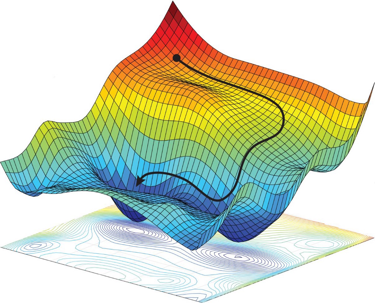
Searching for the best alignment by testing all combinations of alignments within a range will find the best alignment, but it is not the most efficient approach. One optimization we made was a greedy algorithm that shifted the image in the direction that gave it the best score, either left, right, up, or down. It would continue picking the best direction until moving in all possible directions resulted in a worse score. We can think of this approach like how a neural network uses gradient decent to train a model. We have a 2D surface of scores, and we have to move along the surface in the direction of the lowest point, until we cannot move any lower.
While this greatly reduces the number of alignments we have to do, it also has its issues. For example, it might not reach a global minima, and instead get stuck at a local minima. To overcome this challenge, we started the alignment from 9 different starting locations (9 points in a square grid). The run that resulted in the best score was selected as the final alignment. This resolved a lot of our issues and ran faster than the naive approach.
Image Pyramid
We also developed an algorithm that further improves the runtime when processing larger images. This is a recursive algorithm which scales the image down by a factor of two each recursive call and then aligns the image based off the displacement of the smaller images. The objective is to do larger, coarse adjustments when the image is small and faster to process, and make smaller adjustments as the image is larger and slower to process.
This algorithm uses the greedy algorithm as its base alignment algorithm. The pseudocode is given below.
def faster_align(chan1, chan2, shift_by):
    if chan1.shape[0] < 400:
        return fast_align(chan1, chan2)

    # divide image size by 2
    chan1_small = transform.resize(chan1, chan1.shape/2)
    chan2_small = transform.resize(chan2, chan2.shape/2)

    # recurse
    faster_align(chan1_small, chan2_small, shift_by)

    # use alignment from smaller img to help align current size
    amount = shift_by.pop()
    shift_scaled = amount * 2
    adjusted_chan1 = apply_transform(chan1, shift_scaled[0], shift_scaled[1])
    return fast_align(adjusted_chan1, chan2, shift_by)
Evaluation
This table shows the algorithm performance results on 3 different scales of images with each alignment algorithm.
| Alignment algorithm | 300 x 300 px | 750 x 750 px | 1500 x 1500 px |
|---|---|---|---|
| naive | 4.3 s | 151 s | 2832 s |
| greedy | 3.1 s | 44 s | 342 s |
| greedy + image pyramid | 2.7 s | 29 s | 231 s |
As seen from the performance results above, the greedy + image pyramid algorithm performed the best across all ranges of images that we tested. It performs 10 times better than the naive approach on the largest image sizes with very similar alignments.
We also notice that as the image width doubles, the time increases dramatically. This is to be expected because the algorithms are dependent on the size of the input, which is O(n^2) where n is the image width. Note that we didn’t test on 3000 pixel images because it would simply take too long (approximately 26 hours for the naive algorithm)!
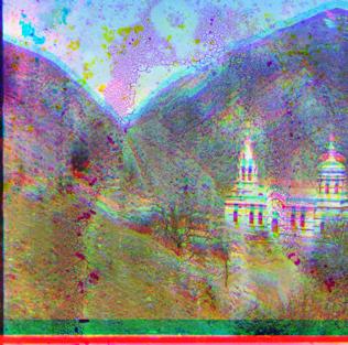
Alternative Alignments - Sobel & Canny Edge Detectors
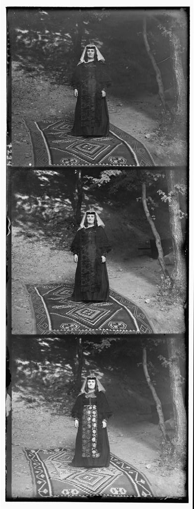
The performance of our alignment algorithms worked very well on the majority of images. Only 3 of the 13 images we tested on with the greedy algorithm resulted in a poor alignment. One example is given below. This image had a stain on the original negative, which we suspect prevents proper alignment just by comparing the RGB values.
We hypothesized that looking at edges or gradients in an image might result in a better alignment. After separating the image into R, G, B arrays and cropping, we applied an edge detection filter to each channel and found the best alignment. Then we can applied the same alignment to the original image.
The filters we tested were the Sobel and Canny filter. The Sobel filter convolves (multiplies each pixel by) a 3x3 kernel (matrix) of weights over an image. The new value of each pixel becomes the sum of the weights of the kernel multiplied by the corresponding values in the image. We used the cv2.sobel() implementation in openCV instead of building it ourselves. A good explanation for these filters can be found here.
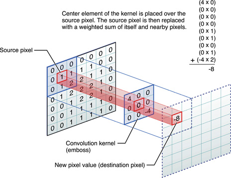
Pictured above: Kernel convolution operation
The Sobel filter did not yield satisfying results and had poorer alignment on all images.
On the other hand, the Canny edge detector builds off of the gradient computed by the Sobel filter and defines harder edges. The output pixels are either 0 or 1. The algorithm takes a lower and upper threshold for connecting the edges, which are manually defined (you can read more about it here) Again, we used cv2.Canny() for this operation.
Evaluation
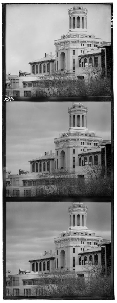
Here are pictures of the Canny edge detection and the resulting alignment.
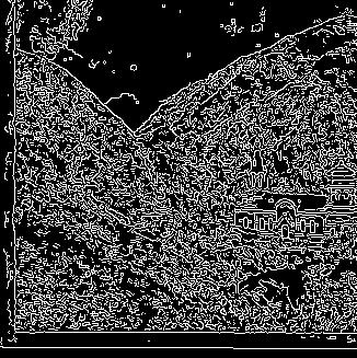
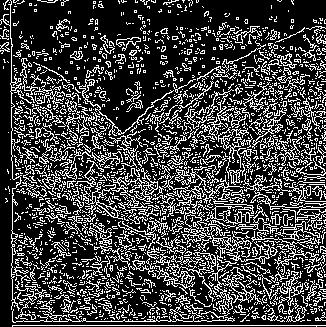
Success! It properly aligned the image when the greedy algorithm failed. However, for most other images, it was worse than the greedy algorithm. We suspect that edge detection depends on what is in the image. For example, it might perform better on a picture of a box, rather than a picture of a fuzzy carpet, because the edges are more defined. We decided not to continue further in this direction, but it was definitely good information.
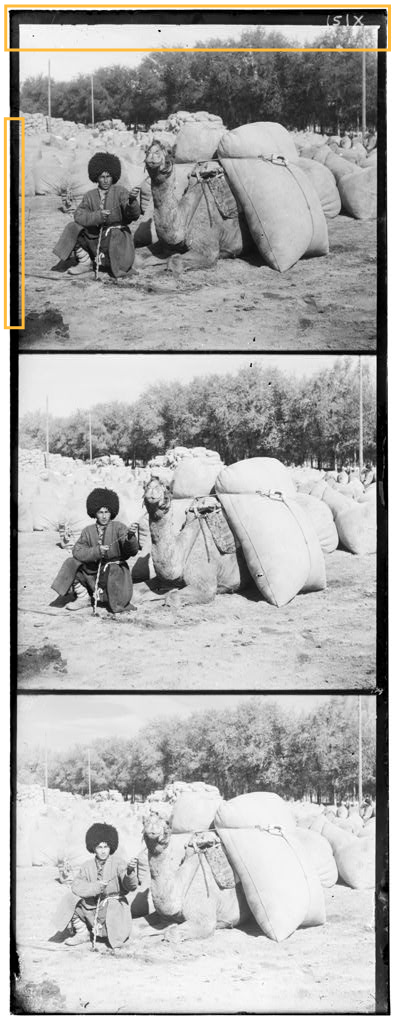
Automatic Cropping
From the single-scale implementation we noticed that the edges were distorting our image alignmenet.
Therefore one of our extra features was to automatically crop out the outer black border on the side of the images.
Consider the following image with the borders we want to get rid of squared off in yellow.
Implementation
Our cropping algorithm tries to find four different borders (top, bottom, left, right) in each of the three images. We know that these borders will have an abnormal density of very dark pixels.
To find the top border we search from the top of the image and if we see a row that has 1/3 of their pixels being very dark < 0.1 we say that row is part of a border. We continue this process until we get inside the image to find the innermost row of a border
    # Blacktop will have the index of the last row of the border
    for i in range(0, int(len(image) / 4)):
        if num_black_pixels(image[i]) > (len(image) / 3):
            black_top = i #A row of the border
To find the bottom border we can search from the bottom instead and work our way towards the center.
    for i in range(len(image) - 1, int(3 * len(image) / 4), -1):
        print(i)
        if num_black_pixels(image[i]) > (len(image) / 3):
            black_bottom = i
To find the left and right borders we simply rotate the image 90 degrees and apply the same process.
black_top, black_bottom = get_black_top_bottom(image)
black_left, black_right = get_black_top_bottom(np.rot90(image))
Then to crop we can simply take these indexes as the new indexes.
return image[black_left:black_right, black_top:black_bottom]
Evaluation
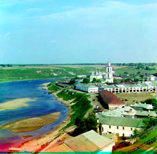
When we run this script with the camel image we notice a large improvement over not cropping out the borders.
This is one of the images where it happens to work very well. However, in some images not all borders are of similar length or black pixel density.
As we can see from this example there are some remnants of the border at the bottom of the image. This could be improved by being more aggresive with what we cut off. However, that would sacrafice being able to view the entire image (in this case the bottom pieces of grass).
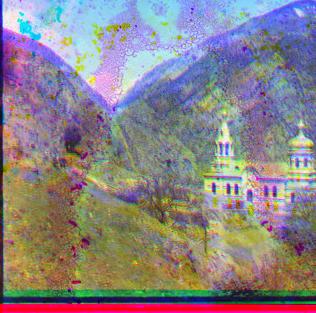
Automatic Contrasting
We also noticed that the images we were producing were quite flat and lacked depth in color.

Image 7: Traditional painting with no automatic contrasting applied.
Take Image 7, a paiting that looks flat in terms of color. No single color pops out and the resulting image feels muted. To help combat this, another feature we implemented was an automatic contrasting algorithm to help increase contrast in the images.
Implementation
def auto_contrast(img):
    p5 = np.percentile(img, 5)
    p95 = np.percentile(img, 95)

    A = [[p5, 1], [p95, 1]]
    B = [0, 1]
    X = np.linalg.inv(A).dot(B)

    for x, row in enumerate(img):
        for y, pixel in enumerate(row):
            for i in range(3): # For each color channel
                img[x][y][i] = X[0] * img[x][y][i] + X[1] # Ax=B

                # Correct pixels outside of valid range [0,1]
                if img[x][y][i] > 1:
                    img[x][y][i] = 1
                elif img[x][y][i] < 0:
                    img[x][y][i] = 0

    return img
The idea behind automatic contrasting is to increase the range of color values in the image. For example, some image may only have 245 as its largest and 10 as its smallest color values. First we can change each of those pixels color chanel values to 255 and 0 respectively. Then, we can scale every other value to take advantage of the increased color range. Note that in our implementation we save rgb information as floats on a [0,1] scale instead of [0,255].
Equation (1): 1 = a * maximum + b
Equation (2): 0 = a * minimum + b
To find the trasnformations needed, one can solve equations (1) and (2) for a and b. In other words, these two equations describe the required transformations to push the maximum color value to 1 and the minimum to 0.
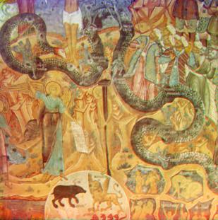
Image 8: Traditional painting with min/max automatic contrasting applied.
Equation (3): 1 = a * p95 + b
Equation (4): 0 = a * p5 + b
As you can, the similarity between these two images is high. In fact, there may be no discernable differences between the two. After a few iterations, we found it was better to use the 95th and 5th percentile single chanel color values. This has the effect of increasing the color range, i.e. increasing the contrast, even more than when using maximum and minimum values. This change is reflected in equations (3) and (4).
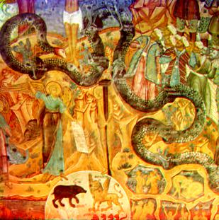
Image 9: Traditional painting with 95/5 percentile automatic contrasting applied.
Image 9 reflects the best version of our auto contrast algorithm. In this image, colors pop and the image becomes more interesting to look at.
Final Evaluations
Below are a few side by side comparisons of our algorithms running on various images.
| Original Image Stack | Auto Align & Auto Crop | Auto Align, Auto Crop, & Auto Contrast |
 |
 |
 |
 |
 |
 |
 |
 |
 |
 |
 |
 |